Let’s try out Julia programming language
As forewords, I have never tried Julia programming language before but I’ve read a couple of headlines about it and they have piqued my interest on the subject. The main motivations to get into the language for me are
- Julia seems to be gaining some momentum in both the programming and especially data science community.
- Even as Julia is dynamically typed it has some static typing going on by enabling the programmer to declare a type if it makes the code easier to understand. This is akin to Python’s type annotation though it seems a little bit more powerful. There is lengthy documentation about this at docs.julialang.org/en/v1/manual/types/. One very definite upside I’ve learned is that you can only subtype abstract types and extending a concrete type is not possible, as a Spring framework user this warms my mind a lot ;) !
- The benchmarks seem to indicate it’s much faster than the main competition Python. This is due to the fact the language is compiled to native code using LLVM.
- You can utilize Python packages.
- I have some background with MatLab and similar plotting stuff seems to be the forte of Julia.
This post is mostly about plotting as it was the main motivation for me to get into Julia language. I’ll try to do the same kind of stuff I did with MatLab with Julia. This means scripting some plotting and I won’t delve into the finer points of e.g. building server-side software.
So if you want deep knowledge and insight into Julia as a language this is not the blog post for you, but if you just want to know how to display some data and setup your own Julia environment please do continue.
Okay how to install this thing
Well let’s google it. The page julialang.org/ is the home page and it has a big download button. Straight away the installation is a bit bare-bones since it’s just a tar-package (mind you I’m using Linux based system) and not some fancy installer or CLI-tool. After I’ve added the extracted bin folder to my PATH it’s time to take the first sip with the repl.
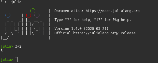
Super! I now have a fancy calculator that seems to be even calculating correctly! After some 20-20 hindsight I can say there is some important information already displayed in the welcome ASCII-art, mainly the ]-mark. This is the way to access Julia package manager for adding dependencies. Also with hindsight using activate <env_name> with the package manager allows you to create python like virtual environments to contain your packages within your project.
So far so good, but I’m one of those guys who likes IDEs especially when learning new languages. The Julia homepage has a nice list of supported and familiar editors and IDEs. But why use something you already know? Let’s go all-in with new stuff and select Atom editor with JUNO plug-in. Ok yes, part of the reason selecting Juno was that it looked cool in screenshots at junolab.org. The installation was quite straightforward as Atom had a .deb-package and after installing it I just needed to add the uber-juno plug-in with atom’s built-in tools. Now I had all the tools in place, time to start coding.
What to do
As said I have some background with MatLab and wanted to do some visualizations as they seem to be the strong point of Julia. So what data to visualize, something current…surprise surprise let’s use COVID-19 data. Basic status data can be acquired from api.covid19api.com using REST calls. So basically to get day to day confirmed cases from Finland issue GET call to api.covid19api.com/country/finland/status/confirmed and you get an array of the following json objects
{
    "Country": "Finland",
    "Province": "",
    "Lat": 61.9241,
    "Lon": 25.7482,
    "Date": "2020-03-31T00:00:00Z",
    "Cases": 1418,
    "Status": "confirmed"
},
After some intensive document reading I found out that I had to add some additional packages to my Julia environment
| Package | Purpose |
|---|---|
| HTTP | To make HTTP calls |
| JSON | Json tools for e.g. parsing |
| Plots | Basic plotting support |
| StatsPlots | Extended plotting support e.g. DataFrames support |
This is achieved with the package manager in the REPL by first issuing the ]-character and then just "activate <env_name>" and then "add HTTP" and so on. This is quite handy, I especially like that the package manager is baked into the REPL instead of being a completely separate tool. Now for some basic coding
using HTTP, JSON, Plots, StatsPlots

resp = HTTP.get("https://api.covid19api.com/country/finland/status/confirmed")
str = String(resp.body)
jobj = JSON.Parser.parse(str)
So what I do here is first issue the HTTP get call to fetch the data from the REST API and then read the body to a string from the stream. Json parsing is quite simple and it produces a dict object. Let’s see what it looks like
println(jobj[0])
>>>
BoundsError: attempt to access 65-element Array{Any,1} at index [0]
in top-level scope at finland_confirmed.jl:6
in getindex at base/array.jl:787
Buggers! I should have seen this coming, as with MatLab in Julia indexes start from 1!!!
println(jobj[1])
>>>
("Lon" => 0,"Status" => "confirmed","Lat" => 0,"Date" => "2020-01-29T00:00:00Z",
"Cases" => 1,"Country" => "Finland","Province" => "")
So now I can easily use the map function to modify it to a format suited for my needs.
cases = map(x -> get(x, "Cases", 0), jobj)
plot(cases)

savefig("images/cases_simple.png") #Save plot as png image
The map function takes a mapping function and the data to apply the function to. I pass an anonymous function to pick up the Cases field and the data I got from the API call. Now that the data is a nice array of values let’s plot it and see what’s what.
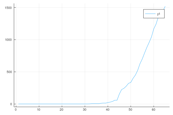
Amazing! I have a basic figure plotted from the data.
More advanced plotting
For trying more advanced plotting I want some more data so let’s add Sweden’s confirmed cases. As a good programmer I want to be DRY so let’s create a function to return the data
function get_country_data(country::String, status::String)
    resp = HTTP.get("https://api.covid19api.com/country/$country/status/$status")
    return JSON.Parser.parse(String(resp.body))
end

finland_confirmed = get_country_data("finland", "confirmed")
sweden_confirmed = get_country_data("sweden", "confirmed")
Couple of things to note. Here is an example on the Julia typing system with the function arguments being typed as Strings. Julia supports string interpolation in perl syntax and contrary to python functions needs an explicit end statement.
The first thing I see is that the data returned for Sweden has a different starting point to Finland’s data so I want to align them by date.
function even_data_sets(list_1, list_2)
    first_date = max(list_1[1]["Date"], list_2[1]["Date"])
    comp = x -> x["Date"] >= first_date
    list_1_m = Iterators.filter(comp, list_1)
    list_2_m = Iterators.filter(comp, list_2)
    return (collect(list_1_m), collect(list_2_m))
end

(even_finland, even_sweden) = even_data_sets(finland_confirmed, sweden_confirmed)
Filtering returns an instance of a filter and to get the actual values you need to collect them, so lazy evaluation is used. Also as the dates are formatted year, month, day we can just use string comparison for the filtering. Okay now lets plot them together
function get_value_array_by_parameter(parameter_name, default_value)
    return x -> get(x, parameter_name, default_value)
end

cases_getter = get_value_array_by_parameter("Cases", 0)
cases_finland = map(cases_getter, even_finland)
cases_sweden = map(cases_getter, even_sweden)

plot([cases_finland, cases_sweden])
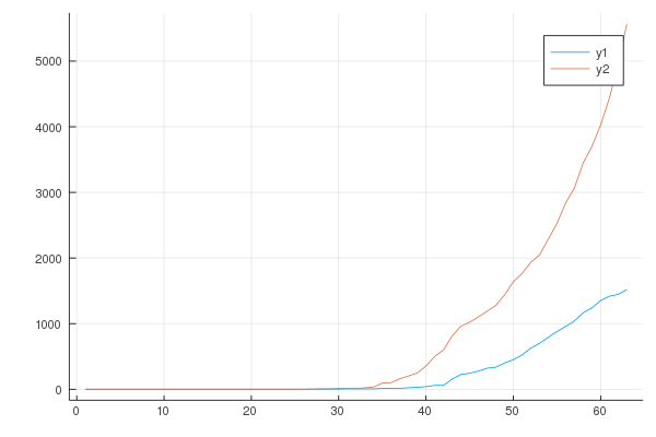
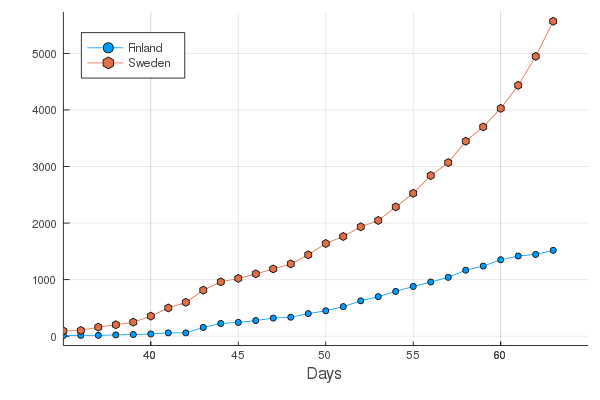
Yeah it’s not much more “advanced” than the first plot, but let’s try to fix that a little by adding some labels limits and dots.
plot([cases_finland, cases_sweden],
    label = ["Finland" "Sweden"],
    legend = :topleft,
    shape = [:circle :hexagon],
    xlabel = "Days",
    xlims = (35,65),
)
Some interesting points on the code
:topleft,:circleand:hexagonare symbols like in Clojure.- The label array. See how there is no comma between the strings? This means the array dimensions are row based as in a first row of a matrix. You can also define a matrix by separating rows with ;-marks, this too is reminiscent of MatLab. The following output elaborates how this works.
julia> [1 2]
1×2 Array{Int64,2}:
 1  2

julia> [1, 2]
2-element Array{Int64,1}:
 1
 2

julia> [1 2;3 4]
2×2 Array{Int64,2}:
 1  2
 3  4
The graphs seem quite “nice” if that kind of term can be used in this kind of a situation. But as with everything GIFs are better so let’s make one
anim = @animate for i in 35:size(cases_finland)[1]
    plot([cases_finland[1:i], cases_sweden[1:i]],
        label = ["Finland" "Sweden"],
        shape = [:circle :hexagon],
        xlabel = "Days",
        xlims = (35,65),
    )
end

gif(anim, "images/progress_fps5.gif", fps = 5)
It’s pretty easy to generate an animation with the helper methods and gif function for saving it with the desired fps.
The @animate is a macro which means that it generates the final code when the program is parsed instead of running it runtime. One great example how this might be useful is from Julia documentation.
macro assert(ex)
    return :( $ex ? nothing : throw(AssertionError($(string(ex)))) )
end

@assert 1 == 1.0
@assert 1 == 0

# This will generate the following final code

1 == 1.0 ? nothing : throw(AssertionError("1 == 1.0"))
1 == 0 ? nothing : throw(AssertionError("1 == 0"))
What is achieved here is that if we would have a simple Assert.assert(1 == 0) call we only have the value of the assertion to play with but now with the macro we have the actual method to assert and we can use it in the error message as well as the valuation.
Summary
Well at least I learned a few things about Julia and it’s features and for me it, seems to be just the right tool when I crave some MatLab plotting (for some reason I haven’t really liked Octave as an alternative). Based on this “try out” it’s hard to say how Julia will fare against e.g. Python in the future but at least the basis seems quite solid with good language features. It’s quite clear that Julia has it’s roots and target audience in the mathematics. This makes it a good alternative for Python in data science with cross-language library support and good performance.
I also want to give a special mention the documentation seems to be excellent as it’s not just a list of functions but also explanations behind the rationals why some decisions have been made. The community behind Julia seems to be very active. The community probably will be the determining factor if there is a future for Julia. For me at least it will be something I’ll try to learn a bit more and add it to my tool belt.